In the consumer lending space, fintech companies have innovated many aspects of the consumer experience. One of the biggest innovations has been the real-time approval of consumers for installment loans with borrowed cash hitting consumer bank accounts in an expedited and highly satisfying way. For those of you not in the business, the loan origination system, as we often call it, provides all of the capabilities to take a credit shopper and turn them into a borrower. To drive this positive consumer experience, fintech lenders rely heavily on real-time credit-scoring processes built into the loan origination system.
Many fintech lenders have advanced innovations using machine learning and data science to develop algorithms that provide a consumer risk score (probability of default) and loan price (interest rate and APR) to the consumer. These algorithms generally ingest consumer credit and financial data to discern the risk of a consumer and provide an appropriately priced installment loan, if possible, given the risk profile.
At the heart of many of these algorithms lies tree-based classification algorithms such as the XGBoost machine learning model, which seeks to classify consumers into risk categories based on their credit and financial profiles. Loan pricing is subsequently determined to generate a profitable loan. Sometimes, for simplicity, loan prices might be determined statically for each risk bucket; for example, all consumers rated a B+ receive and interest rate of 17.99%. Other more sophisticated pricing approaches might provide dynamic pricing.
We used this approach in the past, but in a new effort, we decided to calculate risk and pricing in a manner that aligns more closely to typical fixed income cash flows. In other words, if a consumer installment loan is a series of cash flows, why not calculate the probability of default for each payment and then do a risk adjusted discounted cash flow valuation of the loan that generates a specified profit regardless of risk? In this manner, the loan pricing accounts for the risk of each cash flow and all loans could be targeted to achieve our profit target with interest rates increasing as risk increases.
This approach evolved from research that one of our data scientists did when examining credit risk pricing models and discovered previous academic research using a survival regression algorithm to predict the payment-by-payment probabilities of default for the duration of the loan. A survival regression model is a technique that models the time until an “event” occurs. This family of models is often used in health-care related analysis, where “survival” means exactly that – did the subject survive to the next period. In our case, survival means “no default on payment” in this period, or that the loan value survives to the next payment.
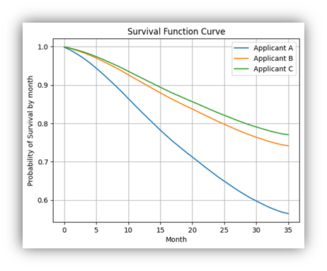
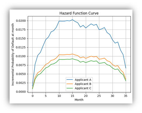
By taking into account credit and financial factors of the individual influencing a potential event of default and a probability of the event of default occurring at payment of the loan, a projected series of default probabilities is generated for the entire loan duration. This series is called the “hazard function curve”. The same risk profile can also be represented in another curve called “survival curve” where each point in the curve denotes the likelihood that a borrower will not default up to the specific point in time.
Here, for three applicants, are the hazard function curves (showing the probability of default at each loan payment) and the survival function curves (showing the probability of no-default up to each loan payment) for a 36-month installment loan.

The two figures display the same three applicants: A, B and C, in two ways, using the cumulative hazard function and the survival function. The higher the forecasted cumulative hazard curve throughout the months, the lower the ending survival probability of the applicant.
The Cox Proportional Hazards algorithm is the specific survival regression method we improved upon to forecast this series of default probabilities throughout the loan term, as shown in the Hazard Function Curve above. Each point on this hazard curve represents the likelihood that the borrower will default on the loan in a specific month, given no default has occurred up to that point. Similar to other supervised machine learning algorithms, we trained the Cox Proportional Hazards model on a dataset comprising historical loan originations, which includes the borrower's financial attributes, loan default status, and time-to-default labels. Once trained, the model evaluates in real-time the default curve (Hazard Function Curve) for a prospective borrower based on their financial attributes, utilizing the predictive power learned from the model features.
The remaining loan origination process requires only fundamental financial analysis to price the loan based on the modeled risks. By applying this resulting default curve to a series of loan payments, we construct a risk weighted cash flow series for the consumer loan. With that series of expected value cash flows, we apply interest rate expenses using a forward curve: In our case, we use the SOFR 1-month forward curve plus our cost of capital spread. We leave a target variable to flex for our interest margin, which iteratively solves (we use an optimization function) to reach the targeted Net Present Value of the loan, which also factors in all origination costs, servicing costs and capital lent to the borrower.
Reference: https://t.co/dkRCobwfts


No comments:
Post a Comment