Unveiling the Enigma: Contrasting Consumer Cash Reserves with Escalating Credit Card Delinquencies

 

A recent analysis sheds light on the intriguing interplay between burgeoning consumer cash reserves and the surprising surge in credit card delinquencies. Despite the Federal Reserve’s reports revealing a remarkable 2.5x increase in cash holdings for the bottom 50% of households, a deeper dive into Transunion’s credit data exposes an unexpected trend in delinquency rates among recently issued credit cards.

Visualizing the Cash Peak:

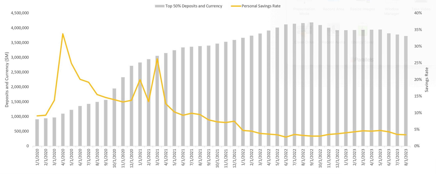
Illustrating the ascent and descent of consumer cash, a Federal Reserve chart showcases the savings rate versus currency and checkable deposits for the top 50% of U.S. households. Notably, cash holdings peaked in September 2022, and while a decline is underway, the rate of decrease suggests a prolonged period before reaching pre-COVID levels.

Delving into Credit Card Delinquencies:

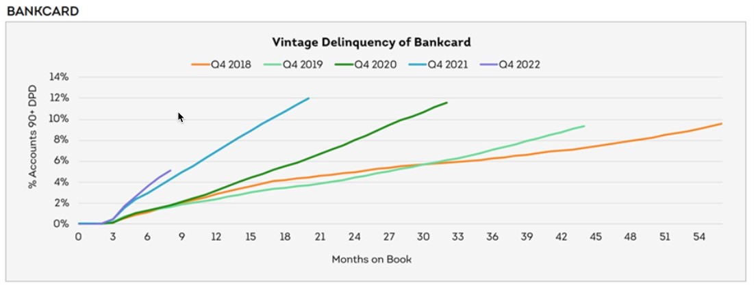
Contrary to expectations, Transunion’s October 2023 report unravels a concerning pattern in credit card delinquencies, particularly among recent issuances. The analysis, organized by vintage (issuance date), indicates a noteworthy acceleration in delinquency rates over shorter periods. Notably, the most recent vintage (Q4 2022) surpasses the pace of all its predecessors.

Savings Rate vs. Currency and Checkable Deposits Top 50% of US Households. Source: Federal Reserve, 2023

Analyzing the Discrepancy:

The conundrum arises – why are credit cards experiencing escalating delinquencies despite consumers holding substantial cash reserves? Several factors contribute to this apparent paradox. The Federal Reserve’s data, reflecting the bottom 50% of households, conceals the nuanced distribution of cash by wealth. A deeper dive into Transunion’s data suggests that stratifying credit risk tiers may unveil higher and faster delinquency rates among lower-grade credit consumers.

Unwinding Positive Effects of COVID Economics:

The favorable effects of COVID-related economic stimuli, such as increased wages, stimulus packages, newfound credit availability, and savings from stay-at-home orders, are now unwinding for lower credit tiers. This segment had the opportunity to spend more and accumulate debt during the pandemic, with banks readily extending new credit accounts. However, as the economy reverts to normalcy, these consumers face regular demands on their cash, leading to a resurgence of credit card bills with historically high-interest rates. Consequently, the combination of heightened financial commitments and mounting credit card debt is fueling a surge in delinquencies, despite the apparent abundance of cash.

In unraveling this financial paradox, it becomes evident that the intricate dynamics of consumer behavior and economic shifts necessitate a comprehensive understanding for stakeholders in the financial landscape.

Reference: https://shorturl.at/puDY7

 Finance

Decoding Consumer Balance Sheets: A Deeper Dive Beyond Savings Rates

 

Navigating the landscape of consumer finance, especially in the realm of excessive debt, prompts questions about the financial robustness of consumers and its potential impact on economic trends. In the post-COVID era, media discussions often revolve around the consumer savings rate, a metric influenced by stimulus measures and changing consumption patterns. However, a recent revelation, supported by alternative data points, challenges conventional perspectives on consumer finances. This analysis delves into the nuances of consumer balance sheets, exploring the interplay between savings rates and the substantial cash build-up in checking accounts.

Alternative Data Insights:

While the savings rate serves as a valuable indicator, it falls short in revealing the depth of cash accumulation. Contrary to widely reported savings rates, a closer look at the Federal Reserve’s Currency and Checkable Deposits data uncovers a more robust and sustainable financial position for the average US consumer. Comparing the cash availability evolution for the Bottom 50% and Top 50% of households reveals a significant uptick, with the former experiencing a 2.5x increase since January 2020 and the latter boasting a more substantial 3.5x surge.

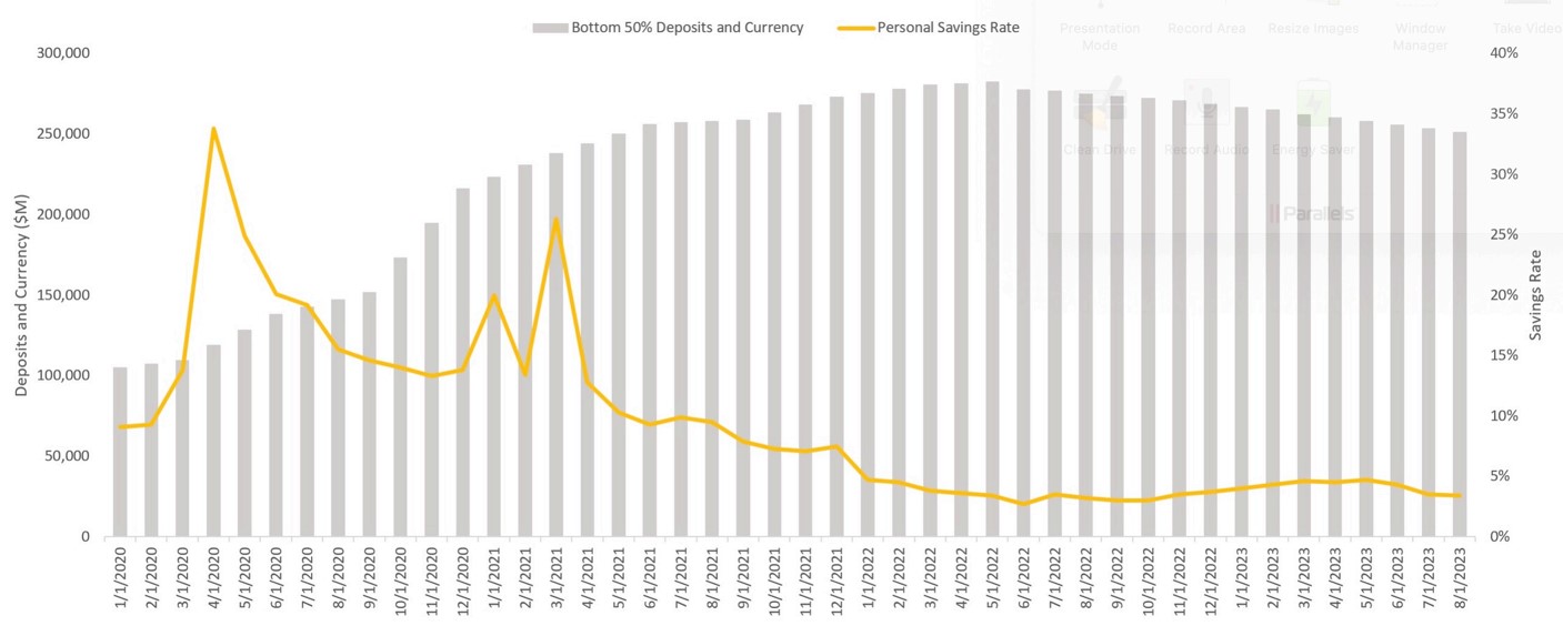
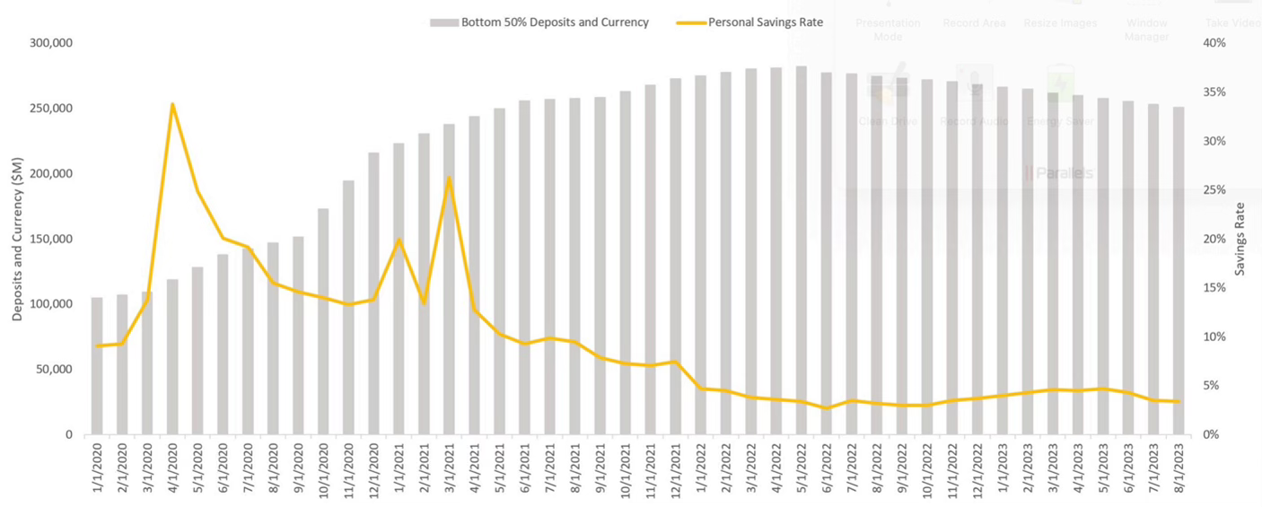
Savings Rate vs. Currency and Checkable Deposits Bottom 50% of US Households

Charting the Course:

The provided charts depict the evolution of Currency and Checkable Deposits for both household groups. Notably, both segments began utilizing their accumulated cash, with the Bottom 50% initiating consumption in June 2022 and the Top 50% following suit in October 2022.

Average Consumer Balance Sheets:

Analyzing these data points underscores the resilience of the average US consumer balance sheets, with ample cash reserves and a prolonged trajectory before returning to pre-COVID levels. However, the sustainability of these balances varies by wealth decile, with wealthier households demonstrating a more protracted cash preservation period.

Erosion of Cash and Wealth Disparities:

It is crucial to acknowledge that these observations represent averages across all households, and the erosion of cash will likely manifest from the bottom up. The bottom 50% has already experienced negative growth, contrasting with the top 50%, signaling potential disparities in the impact of economic shifts. Less affluent households may face recessionary pressures while the broader economy remains relatively stable.

Forecasting Economic Trends:

While consumer balance sheets are not projected to be a significant driver of economic slowdown in the short term, factors like hiring trends, wages relative to inflation, and industrial output are expected to play more substantial roles in shaping the economic landscape. The intricate dynamics of wealth distribution and consumer behavior necessitate a comprehensive understanding for accurate forecasting of a recession or a “soft landing” scenario in the coming years.

Reference: https://tirabassi.com/

Unlocking Synergies: Elevating Data Science with Operations Research Expertise

 **Introduction:**

Who’s on a quest to develop advanced data science capabilities? One of my analytics team’s strategic expansion brought together diverse talents in statistics, applied math, and engineering. This case study explores the integration of operations research, fostering collaboration and knowledge diversity within analytics.

**Objective:**

Our primary goal was to blend diverse skill sets, creating an environment conducive to innovative problem-solving. While the envisioned integration remained a future prospect, immediate focus shifted to operations research for its promising prescriptive capabilities. 

**Operations Research Focus:**

Econometrics was another area if interest for time-series analytics, but operations research, tailored for data science programming and extensive datasets, emerged as a focal point. Excelling in solving objectives within specified constraints, it offered optimal solutions that set it apart from traditional machine learning models.

**Prescriptive Analytics vs. Predictive Analytics:**

Distinguish prescriptive analytics (operations research) from predictive analytics (machine learning). The former provides optimal solutions based on defined constraints, while the latter predicts outcomes based on historical data.

**Transportation Example:**

In a transportation scenario, predictive models analyze historical data for efficient routes. Operations research, however, prescriptively determines the least-cost path based on constraints, suggesting routes not traveled before. One other aspect of operations research and linear programming models is that they also handle revenue and expense variables quite well.

**Methodology and Insight:**

While both approaches may lead to similar conclusions, their methodologies diverge significantly. Predictive models embrace uncertainty, offering likely outcomes, while operations research precisely calculates optimal solutions, evaluating all possible choices.

**Data Science Synergy:**

Understanding this nuanced difference empowers an analyst or data scientist to approach problem-solving flexibly. Predictive models shine in uncertainty, providing choices based on learned experiences. Operations research excels with known inputs and complex combinations, delivering reliable solutions.

**Conclusion and Future Prospects:**

This case study illuminates the ongoing journey in cultivating a collaborative data science environment. As the capabilities of a team evolve, the prospect of adding talents like the previously mentioned econometrics, which excels in time-series forecasting, holds the promise of elevating capabilities to tackle even more complex challenges. Unleash the potential of data science synergy with operations research expertise! 

 🌐📈 #DataScience #OperationsResearch #AnalyticsSynergy #PrescriptiveAnalytics #PredictiveAnalytics #CaseStudy

 Reference:- http://tirabassi.com/

Unlocking Value Creation: The Power of Lifetime Customer Value in Operational Execution

You might see it in various places as CLV (Customer Lifetime Value) or LTV (Lifetime Value). Lifetime Customer Value, or LCV, is what I call this metric. Fairly interchangeable in my experience, people who use these metrics regularly will know what you mean when you refer to any one of them. LCV’s compact measurement of the value of an individual customer unit is powerful. It’s something that I have been using for years and would like to share some insights into it.

Conceptually, LCV can be calculated as the net value of a customer over their lifetime. In theory, if you calculate it to a net value including allocated overhead costs for every single customer and then summed all of those individual values up, you should be very close or equal to the enterprise value of a business calculated in a discounted cash flow. These two things (Sum of LCV and DCF EV) equate because the LCV is basically taking the net present value of each individual customer’s cash flow, and when summed up, it should equal the net present value of the company’s cash flow. As mentioned, this assumes you calculate LCV on a net basis with accurate allocation of overheads.

If you look at it from the other direction, you could say that LCV equals EV divided by all active customers. Cable television companies often use (at least I think they still do) the EV divided by active customers to derive a value per subscriber metric for valuation purposes. This is a very easy way to examine the relative strength of the individual subscribers across companies by comparing the relative value per subscriber between companies.

The importance of these equalities is that LCV, as an operational metric usable in all areas of the organization, is tied to value creation for the entire business. If marketing pushes Customer Acquisition Cost (CAC) down, then LCV goes up, and the business should gain value. If the cost of goods sold goes up, then LCV goes down, and so does the value of the business. If an organization embraces this metric, they can push shareholder value creation alignment into many corners of a company.

When it comes to LCV, one of the main areas of focus in most cases, I find, is CAC. CAC can be volatile, especially in a world of digital marketing, where competitive forces can turn against you and make marketing very expensive in short and even sustained periods of time. As a result, if you have sticky pricing and overall operating expenses over the course of a year, CAC tends to be the part of LCV that causes the most fluctuation.

When it comes to marketing, CAC does this in two main ways. The marketing expense can fluctuate in or out of your favor, which drives LCV up or down. But given that marketing fluctuations can also translate into higher or lower customer acquisition counts, the LCV can compound its impact on the overall valuation – the sum of the LCVs as described above.

The two-by-two below illustrates the concept at a very high level.

Another area of interest is LCV as a contribution calculation before overhead versus LCV as a net calculation after overhead. The table below shows the differences between the two calculations at a high level.

I already touched on the net calculation and how it is connected to EV. The contribution calculation gives you LCV down to the contribution margin level, which is to say LCV-Contribution is the lifetime customer value that can be used to pay all overhead and financing costs of the company. This is particularly useful if the organization has steady overhead costs that don’t increase quickly with the customer base. It gives the business operators a sense of how many customers they can add to the business on a marginal basis profitably. It allows the operators to take aggressive approaches to CAC and Cost of Goods/Services because every customer with some value at the contribution level will drive growth in EV. With that said, such an approach would lower net LCV over time as lower contribution clients would dilute the average LCV.

To sum it up, Lifetime Customer Value (LCV) is a powerful tool that goes beyond just numbers. It tells us the long-term value of each customer and how it connects to the overall value of a business. By paying attention to LCV, companies can make smart decisions that impact everything from marketing costs to the value of the entire business. In the fast-paced world of digital marketing, where things can change quickly, understanding and using LCV gives businesses a reliable way to plan for the future. The simple matrix and the difference between net and contribution calculations show how flexible and useful LCV can be. So, as businesses delve into LCV insights, they can uncover new ways to improve their strategies, build better relationships with customers, and set the stage for lasting success.

Reference: https://shorturl.at/xyPX0

An AI Crystal Ball? How We Predict Future Outcomes Using a Temporal Fusion Transformer Model

Our data science and analytics teams handle and apply lots of data for insightful decision-making. Last year, I presented the data science team with a challenge: use historical data to predict a key business driver for each of the next 8 periods. We wanted to have a data-driven preview of what we might see in the in each of the next eight periods so that we could anticipate the actual outcome and make better decisions with a an eight-period.

The data science team went to work researching ways we could do this and tested a few different methodologies. We have lots of input data from our own and public sources to feed any model we wanted to test, which worked well for us. With that said, we had low expectations about finding a predictive model that produced anything reliable.

Testing different algorithms is always our approach. For the semi-technical readers, before settling on Temporal Fusion Transformer (TFT), the algorithms we tested included ARIMA, VAR, GARCH, ARCH models (univariate), Prophet, NHits, and Nbeats. TFT is an attention-based deep learning neural network algorithm. Using a mix of inputs, it produces a forecast over multiple periods in a future time horizon that you can determine. You can predict days, weeks, months quarters (really any interval is possible) into the future. Your choice.

The picture below shows the concept of how TFT works.

Source: Bryan Lim, Sercan Ö. Arık, Nicolas Loeff, Tomas Pfister. “Temporal Fusion Transformers for interpretable multi-horizon time series forecasting.” International Journal of Forecasting. Volume 37, Issue 4, October–December 2021, Pages 1748-1764.

A continuous improvement process best describes how we developed and continue to refine the model. It’s a never ending process of improvement, as a true crystal ball is never achieved.

These are the four stages of development we went through after choosing TFT as our algorithm:

• Stage 1a: Selecting all logical observed inputs and test how they drive the model. We started with over 100 and the final model only used 20. Go to Stage 1b as needed.
• Stage 1b: Refining the time intervals of the observed inputs. Since the inputs might come in varying time intervals (daily, weekly, monthly and quarterly, etc…), we needed to find methods to standardize them. You should choose an interval that matches the decision-making forecast you are producing, if you can. Go back to Stage 1a as needed.
• Stage 2: Model iteration and improvement. Complete back testing. Examine early predictions. Go back to Stages 1a and 1b as needed. At this point, you have probably settled on one or two of the most promising algorithms.
• Stage 3: Begin using in production and comparing predictions to the future periods as they unfold. Learn and refine by going back to any previous stage as needed.
• Stage 4. Continuous improvement loop. Write long-term road map. Test new inputs as they are presented. Continuous scrutiny of the predictions against what actually happens – learn and make changes by going back to any previous stage as needed.

Note that at any of the stages of development, you can use a TFT encoder decoder to measure the importance of different inputs in the algorithm to learn which ones have the most impact on your prediction.

Below are the results of our model. The orange line is the actual result of the key driver and the blue line is the prediction of the key driver that was made 8 periods ago. The area to the right without the orange line is the next 8-period forecast. So, at Period 19, we can use the blue line forecast to take action based on what Periods 20-27 tell us. When we reach Period 20, we evaluate the updated forecast and we make a decisions accordingly for the future periods. This way, we have a rolling 8-period prediction/decision cycle.

As you can see the model has been refined to a level that it makes useful predictions and handles volatility of the prediction with some reliability. Right now, we don’t use this to predict the future down to the exact number, which would be ideal, but we use it for a directional understanding of where things are headed so we can make better decisions at the current decision point.

Key Consideration For SaaS (or Any Recurring Revenue) Financial Models

In SaaS, decoding revenue dynamics is pivotal for pushing the business forward. Let's talk about the elements of financial modeling tailored for SaaS companies:

1. Revenue Insights:

MRR (Monthly Recurring Revenue): This quantifies the predictable monthly revenue, offering immediate insights into short-term revenue trends. In my experience, I build monthly forecasts and report on the business against the forecast monthly. Having a predictable MRR with less than 1% variance to the rolling 90-day forecast is achievable and ideal. (Of course, early in the business these variances could be higher.)

ARR (Annual Recurring Revenue): An annualized view of MRR, guiding long-term planning and providing a comprehensive overview of revenue trajectory. Often ARR is used to give investors a sense of how much revenue the business has on the books that will repeat for the following year. This gives comfort to investors who see this as a baseline of revenue helping fund the company. Personally, I think contracted backlog is a more interesting way to look at this same element of SaaS, but I will cover that another day.

Churn Rate (aka cancellation rate): Measuring customer subscription cancellation, influencing MRR and ARR. Managing and reducing churn is crucial for cost-effective customer retention. Churn has two important modeling conventions that you should consider: first, does your cancellation rate change with the age of the client or contract. This is heavily influenced by the contract duration, but if you have no duration, this is an important factor to consider. Second, when modeling, it is often easier to model client counts as retention, which is (1-churn%). Always be sure that you are applying this correctly as there is a difference between churn-to-date and churn since the last period.

2. Cost Projections:

COGS (Cost of Goods Sold): Direct costs related to delivering the software service, impacting gross margin and signaling operational efficiency. Accurate forecasting is vital for profitability projections. Cloud services and direct IT support of software delivery and up-time fit into this bucket.

Operating Expenses: Day-to-day operational costs affecting operating margin and overall profitability. Monitoring ensures business efficiency and agility. This includes more typical overheads like rent, sales and marketing costs, R&D and management.

3. Customer-Centric Metrics:

CAC (Customer Acquisition Cost): Evaluating the average cost to acquire a customer. Discrepancies between CAC and customer LTV (Lifetime Value) indicate marketing or sales process inefficiencies. CAC should include all sales and marketing costs, including sales overhead for things like a CRM software, pre-sales scheduling and sales management. If you leave these items out, you are really looking at marketing acquisition cost. It’s useful in some cases to do this, but CAC, especially when you are running dynamic LTV analysis.

Retention Rate: Depending on how you want to use this, it could be a very granular financial model component. Otherwise, it can simply be the percentage of retained ARR over a specified period. The latter example again is an important metric to help convince investors you have a stable source of revenues.

LTV (Lifetime Value) aka LCV (Lifetime Customer Value): One basic approach is to calculate this as total gross profit from a customer throughout the lifecycle of the client. Personally, I like to be very granular with this and I use specific components of the above for the analysis: -CAC, +churn adjusted revenues, -churn adjusted COGS = LTV Contribution and -allocated overhead = Net LTV. In addition to the final LTV values, I look at the following ratios: LTV Contribution to CAC and LTV Net to CAC. Note: Churn adjusted revenues and expenses are very useful when you have client with changing cancellation rates over time. Pro tip: You can also look at this by subscription cohorts if you sign up a lot of contracts each month.

4. Financial Health Analysis:

Cash Flow: Tracking cash movement for informed management of working capital and expense management.

Break-Even Analysis: Predicting profitability by determining the sales volume needed to cover costs. Essential for strategic pricing and sales strategies. In this area, it’s useful to look at the count, value and consistency of new contract additions in the forecast to determine when the business becomes profitable.

Understanding these components offers a complete view of the current and future operation, empowering leaders to make informed decisions aligned with growth objectives. The interplay of revenue insights, cost projections, customer-centric metrics, and financial health analysis forms the bedrock for a robust SaaS financial model.

Unraveling the Complexities of Consumer Balances Sheets Post-Covid

As discussions go round and round regarding the potential impact of consumer finances on an impending recession or a more gradual "soft landing," recent media narratives have brought attention to a remarkable surge in the savings rate following the COVID-19 pandemic.

While the savings rate serves as a useful metric, providing insights into where consumers are directing their excess cash, it falls short in offering a nuanced understanding of the actual cash buildup. Recently disclosed data has ushered in a paradigm shift, challenging preconceived notions about consumer savings. The revelation suggests that consumers have saved more cash than previously estimated, with reported savings rates reaching 15.4% in 2020 and 11.4% in 2021—figures that are undeniably significant.

Prompted by this new data report, my focus has been directed towards the Federal Reserve's reporting on Currency and Checkable Deposits, a comprehensive analysis tracking the ebb and flow of cash in checking accounts. This alternative data perspective paints a more optimistic picture of the consumer's financial standing, revealing that the average US consumer is holding multiples of cash compared to pre-COVID levels. This newfound understanding underscores the robustness and sustainability of consumer balances, fueled by higher average savings rates.

Let's explore how Currency and Checkable Deposits have evolved for different segments of the population, particularly the Bottom 50% and Top 50% of households.

Cash and checkable deposits for the bottom 50% of households by wealth. Federal Reserve, 2023.

Cash and checkable deposits for the top 50% of households by wealth. Federal Reserve, 2023.

The charts vividly illustrate the substantial growth in cash availability, with the Bottom 50% experiencing a 2.5x increase from January 2020 to August 2023, and the Top 50% boasting over 3.5x more cash during the same period. Intriguingly, both groups have begun consuming their accumulated cash, a trend that commenced in June 2022 for the bottom 50% and October 2022 for the top 50%.

These data points collectively paint a comprehensive picture, indicating that, on average, US consumer balance sheets remain resilient and robust. The runway for these balance sheets to return to pre-COVID cash levels appears long. However, it's crucial to acknowledge that these are averages across all households, and the sustainability of cash levels varies by the decile of wealth.

In dissecting this narrative further, it becomes evident that the erosion of cash is not uniform and is likely to follow a bottom-up trajectory. This divergence is observable as the bottom 50% experiences negative growth since June 2022, preceding the top 50% that exhibits similar trends from October 2022. The implication is that less affluent households might feel the impacts of a potential recession earlier than their wealthier counterparts.

As we navigate the complex terrain of economic forecasting, it's essential to recognize that while consumer balance sheets play a role, they may not emerge as the primary driver of an economic slowdown. Other economic factors, such as hiring trends, wage dynamics relative to inflation, and industrial output, are anticipated to wield a more substantial influence in shaping the trajectory of the economic slowdown.

Reference: https://shorturl.at/uJLO1